New Project
File > New Project..

New Project
Set the directory name and the subdirectory.
R Markdown
You can write the report with RMarkdown. It can generate HTML, PDF, Word, and PPT documents. Furthermore, math equations can be write with LaTex format.
Find the cheet sheet from Help > Cheetsheets > R Markdown Cheet Sheet
Create your R Markdown!

R Markdown
Add the title and author name.

Setup
Kick the “Knit” button.

Knit
Then you will see the following example.
R Markdown
This is an R Markdown document. Markdown is a simple formatting syntax for authoring HTML, PDF, and MS Word documents. For more details on using R Markdown see http://rmarkdown.rstudio.com.
When you click the Knit button a document will be generated that includes both content as well as the output of any embedded R code chunks within the document. You can embed an R code chunk like this:
summary(cars)#> speed dist
#> Min. : 4.0 Min. : 2.00
#> 1st Qu.:12.0 1st Qu.: 26.00
#> Median :15.0 Median : 36.00
#> Mean :15.4 Mean : 42.98
#> 3rd Qu.:19.0 3rd Qu.: 56.00
#> Max. :25.0 Max. :120.00Including Plots
You can also embed plots, for example:
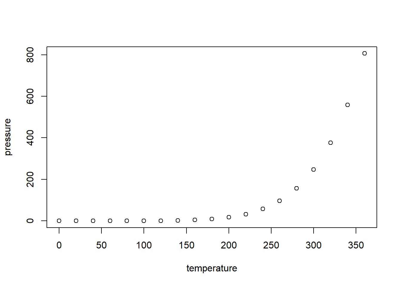
Note that the echo = FALSE parameter was added to the code chunk to prevent printing of the R code that generated the plot.
R Code Chunks
shortcut
Ctrl + Alt + I on Windows
Cmd + Option + I on macOS
Add your R code in code chunk, then R Markdown will run it.
```{r}
summary(cars)
```summary(cars)#> speed dist
#> Min. : 4.0 Min. : 2.00
#> 1st Qu.:12.0 1st Qu.: 26.00
#> Median :15.0 Median : 36.00
#> Mean :15.4 Mean : 42.98
#> 3rd Qu.:19.0 3rd Qu.: 56.00
#> Max. :25.0 Max. :120.00```{r}
x = 5 # radius of a circle
```For a circle with the radius `r x`,
its area is `r pi * x^2`.x = 5 # radius of a circleFor a circle with the radius 5, its area is 78.5398163.
LaTex
Use $ to add math equations in the paragraph.
the acceptance rate in $95\%$ confidence
the acceptance rate in \(95\%\) confidence
Use $$ to add math equations in single or multiple lines.
$$
f_X(x) = {x-1 \choose r-1} p^r (1-p)^{x-r} I_{(r,r+1, \dots)} (x)
$$
\[ f_X(x) = {x-1 \choose r-1} p^r (1-p)^{x-r} I_{(r,r+1, \dots)} (x) \]
$$
\begin{aligned}
f_X(x) = {x-1 \choose r-1} p^r (1-p)^{x-r} I_{(r,r+1, \dots)} (x)
f_X(x) = {x-1 \choose r-1} p^r (1-p)^{x-r} I_{(r,r+1, \dots)} (x)
\end{aligned}
$$
\[ \begin{aligned} f_X(x) = {x-1 \choose r-1} p^r (1-p)^{x-r} I_{(r,r+1, \dots)} (x)\\ f_X(x) = {x-1 \choose r-1} p^r (1-p)^{x-r} I_{(r,r+1, \dots)} (x) \end{aligned} \]
For more information, see Latex in Wiki.
Wrangle with Data
Prerequisite
# install.packages("tidyverse")
library(tidyverse)
#> -- Attaching packages --------------------------------------- tidyverse 1.3.0 --#> √ ggplot2 3.3.3 √ purrr 0.3.4
#> √ tibble 3.0.6 √ dplyr 1.0.4
#> √ tidyr 1.1.2 √ stringr 1.4.0
#> √ readr 1.4.0 √ forcats 0.5.1#> -- Conflicts ------------------------------------------ tidyverse_conflicts() --
#> x dplyr::filter() masks stats::filter()
#> x dplyr::lag() masks stats::lag()Tidyverse contains the packages you may need to use in data science, including ggplot2, dplyr, etc. So you do not need to install them individually.
Data
ggplot2::mpg#> # A tibble: 234 x 11
#> manufacturer model displ year cyl trans drv cty hwy fl class
#> <chr> <chr> <dbl> <int> <int> <chr> <chr> <int> <int> <chr> <chr>
#> 1 audi a4 1.8 1999 4 auto(l~ f 18 29 p comp~
#> 2 audi a4 1.8 1999 4 manual~ f 21 29 p comp~
#> 3 audi a4 2 2008 4 manual~ f 20 31 p comp~
#> 4 audi a4 2 2008 4 auto(a~ f 21 30 p comp~
#> 5 audi a4 2.8 1999 6 auto(l~ f 16 26 p comp~
#> 6 audi a4 2.8 1999 6 manual~ f 18 26 p comp~
#> 7 audi a4 3.1 2008 6 auto(a~ f 18 27 p comp~
#> 8 audi a4 quat~ 1.8 1999 4 manual~ 4 18 26 p comp~
#> 9 audi a4 quat~ 1.8 1999 4 auto(l~ 4 16 25 p comp~
#> 10 audi a4 quat~ 2 2008 4 manual~ 4 20 28 p comp~
#> # ... with 224 more rows?ggplot2::mpg # For more information
Or you can simply call ?mpg if you had already call the library.
Select columns with select()
df <- select(mpg, manufacturer, cty, hwy, class)
df
summary(df)
table(df %>% select(manufacturer, class))
df <- select(mpg, manufacturer, cty, hwy, class)
df#> # A tibble: 234 x 4
#> manufacturer cty hwy class
#> <chr> <int> <int> <chr>
#> 1 audi 18 29 compact
#> 2 audi 21 29 compact
#> 3 audi 20 31 compact
#> 4 audi 21 30 compact
#> 5 audi 16 26 compact
#> 6 audi 18 26 compact
#> 7 audi 18 27 compact
#> 8 audi 18 26 compact
#> 9 audi 16 25 compact
#> 10 audi 20 28 compact
#> # ... with 224 more rowssummary(df)#> manufacturer cty hwy class
#> Length:234 Min. : 9.00 Min. :12.00 Length:234
#> Class :character 1st Qu.:14.00 1st Qu.:18.00 Class :character
#> Mode :character Median :17.00 Median :24.00 Mode :character
#> Mean :16.86 Mean :23.44
#> 3rd Qu.:19.00 3rd Qu.:27.00
#> Max. :35.00 Max. :44.00table(df %>% select(manufacturer, class))#> class
#> manufacturer 2seater compact midsize minivan pickup subcompact suv
#> audi 0 15 3 0 0 0 0
#> chevrolet 5 0 5 0 0 0 9
#> dodge 0 0 0 11 19 0 7
#> ford 0 0 0 0 7 9 9
#> honda 0 0 0 0 0 9 0
#> hyundai 0 0 7 0 0 7 0
#> jeep 0 0 0 0 0 0 8
#> land rover 0 0 0 0 0 0 4
#> lincoln 0 0 0 0 0 0 3
#> mercury 0 0 0 0 0 0 4
#> nissan 0 2 7 0 0 0 4
#> pontiac 0 0 5 0 0 0 0
#> subaru 0 4 0 0 0 4 6
#> toyota 0 12 7 0 7 0 8
#> volkswagen 0 14 7 0 0 6 0Filter rows with filter()
Logic “and”
filter(df, class == "compact", cty < 20)#> # A tibble: 21 x 4
#> manufacturer cty hwy class
#> <chr> <int> <int> <chr>
#> 1 audi 18 29 compact
#> 2 audi 16 26 compact
#> 3 audi 18 26 compact
#> 4 audi 18 27 compact
#> 5 audi 18 26 compact
#> 6 audi 16 25 compact
#> 7 audi 19 27 compact
#> 8 audi 15 25 compact
#> 9 audi 17 25 compact
#> 10 audi 17 25 compact
#> # ... with 11 more rowsLogic “or”
These three are equivalent.
filter(df, class == "compact" | class == "suv")
df %>% filter(class == "compact" | class == "suv")
df %>% filter(class %in% c("compact", "suv"))
filter(df, class == "compact" | class == "suv")#> # A tibble: 109 x 4
#> manufacturer cty hwy class
#> <chr> <int> <int> <chr>
#> 1 audi 18 29 compact
#> 2 audi 21 29 compact
#> 3 audi 20 31 compact
#> 4 audi 21 30 compact
#> 5 audi 16 26 compact
#> 6 audi 18 26 compact
#> 7 audi 18 27 compact
#> 8 audi 18 26 compact
#> 9 audi 16 25 compact
#> 10 audi 20 28 compact
#> # ... with 99 more rowsdf %>% filter(class == "compact" | class == "suv")#> # A tibble: 109 x 4
#> manufacturer cty hwy class
#> <chr> <int> <int> <chr>
#> 1 audi 18 29 compact
#> 2 audi 21 29 compact
#> 3 audi 20 31 compact
#> 4 audi 21 30 compact
#> 5 audi 16 26 compact
#> 6 audi 18 26 compact
#> 7 audi 18 27 compact
#> 8 audi 18 26 compact
#> 9 audi 16 25 compact
#> 10 audi 20 28 compact
#> # ... with 99 more rowsdf %>% filter(class %in% c("compact", "suv"))#> # A tibble: 109 x 4
#> manufacturer cty hwy class
#> <chr> <int> <int> <chr>
#> 1 audi 18 29 compact
#> 2 audi 21 29 compact
#> 3 audi 20 31 compact
#> 4 audi 21 30 compact
#> 5 audi 16 26 compact
#> 6 audi 18 26 compact
#> 7 audi 18 27 compact
#> 8 audi 18 26 compact
#> 9 audi 16 25 compact
#> 10 audi 20 28 compact
#> # ... with 99 more rowsSummary
You can work this way!
mpg %>%
  select(manufacturer, cty, hwy, class) %>%
  filter(class %in% c("compact", "suv"))
#> # A tibble: 109 x 4
#> manufacturer cty hwy class
#> <chr> <int> <int> <chr>
#> 1 audi 18 29 compact
#> 2 audi 21 29 compact
#> 3 audi 20 31 compact
#> 4 audi 21 30 compact
#> 5 audi 16 26 compact
#> 6 audi 18 26 compact
#> 7 audi 18 27 compact
#> 8 audi 18 26 compact
#> 9 audi 16 25 compact
#> 10 audi 20 28 compact
#> # ... with 99 more rowsHomework
Wrangle with ggplot2::mpg and show the result.
Select
manufacturer,year, anddispl.Filter
yearis 1999 anddispl < 2.
Reference solution
#> # A tibble: 234 x 3
#>    manufacturer  year displ
#>    <chr>        <int> <dbl>
#>  1 audi          1999   1.8
#>  2 audi          1999   1.8
#>  3 audi          2008   2
#>  4 audi          2008   2
#>  5 audi          1999   2.8
#>  6 audi          1999   2.8
#>  7 audi          2008   3.1
#>  8 audi          1999   1.8
#>  9 audi          1999   1.8
#> 10 audi          2008   2
#> # ... with 224 more rows
#> # A tibble: 17 x 3
#> manufacturer year displ
#> <chr> <int> <dbl>
#> 1 audi 1999 1.8
#> 2 audi 1999 1.8
#> 3 audi 1999 1.8
#> 4 audi 1999 1.8
#> 5 honda 1999 1.6
#> 6 honda 1999 1.6
#> 7 honda 1999 1.6
#> 8 honda 1999 1.6
#> 9 honda 1999 1.6
#> 10 toyota 1999 1.8
#> 11 toyota 1999 1.8
#> 12 toyota 1999 1.8
#> 13 volkswagen 1999 1.9
#> 14 volkswagen 1999 1.9
#> 15 volkswagen 1999 1.9
#> 16 volkswagen 1999 1.8
#> 17 volkswagen 1999 1.8