TA_class_1212

# S3 method for default
t.test(x, y = NULL,
       alternative = c("two.sided", "less", "greater"),
       mu = 0, paired = FALSE, var.equal = FALSE,
       conf.level = 0.95, …)

# S3 method for formula
t.test(formula, data, subset, na.action, …)

單組樣本

先透過畫圖與敘述統計量了解資料的樣貌。再進行假設檢定的步驟。

boxplot(mpg$cty)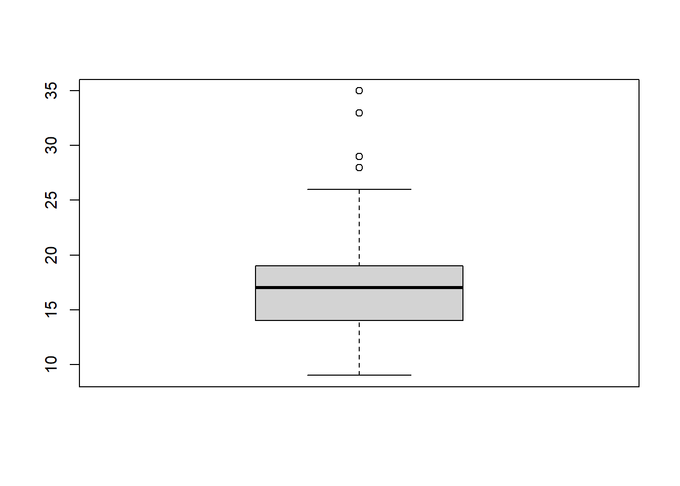

summary(mpg$cty)

#>    Min. 1st Qu.  Median    Mean 3rd Qu.    Max. 
#>    9.00   14.00   17.00   16.86   19.00   35.00

\[ \begin{aligned} \left\{ \begin{array}{ll} H_0: & \mu \geq 20\\ H_1: & \mu < 20 \end{array} \right. \end{aligned} \]

t.test(mpg$cty, alternative = "less", mu = 20, conf.level = 0.99)

#> 
#>  One Sample t-test
#> 
#> data:  mpg$cty
#> t = -11.29, df = 233, p-value < 2.2e-16
#> alternative hypothesis: true mean is less than 20
#> 99 percent confidence interval:
#>      -Inf 17.51069
#> sample estimates:
#> mean of x 
#>  16.85897

hy.cty <- t.test(mpg$cty, alternative = "less", mu = 20, conf.level = 0.99)

hy.cty

#> 
#>  One Sample t-test
#> 
#> data:  mpg$cty
#> t = -11.29, df = 233, p-value < 2.2e-16
#> alternative hypothesis: true mean is less than 20
#> 99 percent confidence interval:
#>      -Inf 17.51069
#> sample estimates:
#> mean of x 
#>  16.85897

t.test() 回傳的資料型態是屬於 list。在 Global Environment 可以見到 hy.cty 是 List of 10，點開來看，可以知道 list 每項的名稱。取值的方式如下:

hy.cty$p.value

#> [1] 3.65265e-24

hy.cty[[3]]

#> [1] 3.65265e-24

hy.cty$conf.int

#> [1]     -Inf 17.51069
#> attr(,"conf.level")
#> [1] 0.99

hy.cty[[4]]

#> [1]     -Inf 17.51069
#> attr(,"conf.level")
#> [1] 0.99

hy.cty$estimate

#> mean of x 
#>  16.85897

hy.cty[[5]]

#> mean of x 
#>  16.85897

兩組樣本

以市區油耗以及高速公路油耗為例。

df <- mpg %>%
  select(cty,hwy) %>%
  gather(cty, hwy, key = "mpg", value = "value")

ggplot(df) +
  geom_boxplot(aes(mpg, value))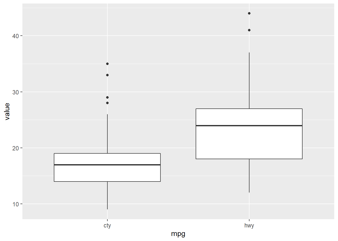

假設兩組樣本皆屬於常態分配的情況下，檢驗兩組樣本的變異數是否有顯著差異。

# S3 method for default
var.test(x, y, ratio = 1,
         alternative = c("two.sided", "less", "greater"),
         conf.level = 0.95, …)

# S3 method for formula
var.test(formula, data, subset, na.action, …)

比如比較市區油耗以及高速公路油耗。

var.test(mpg$cty, mpg$hwy, ratio = 1,
         alternative = "two.sided",
         conf.level = 0.90)

#> 
#>  F test to compare two variances
#> 
#> data:  mpg$cty and mpg$hwy
#> F = 0.51083, num df = 233, denom df = 233, p-value = 3.891e-07
#> alternative hypothesis: true ratio of variances is not equal to 1
#> 90 percent confidence interval:
#>  0.4116158 0.6339708
#> sample estimates:
#> ratio of variances 
#>           0.510835

因為 F-test 的 p-value 小於顯著水準 0.1， 表示兩組樣本的變異數有顯著差異，因此 t-test 假設變異數不相等，設定 var.equal = FALSE。 假如是成對樣本，設定 paired = TRUE， 不是成對樣本，設定 paired = FLASE。

# Paired t-test
t.test(mpg$cty, mpg$hwy,
       alternative = "less",
       mu = 0, paired = TRUE, var.equal = FALSE,
       conf.level = 0.99)

#> 
#>  Paired t-test
#> 
#> data:  mpg$cty and mpg$hwy
#> t = -44.492, df = 233, p-value < 2.2e-16
#> alternative hypothesis: true difference in means is less than 0
#> 99 percent confidence interval:
#>     -Inf -6.2347
#> sample estimates:
#> mean of the differences 
#>               -6.581197

# Welch Two Sample t-test
t.test(mpg$cty, mpg$hwy,
       alternative = "less",
       mu = 0, paired = FALSE, var.equal = FALSE,
       conf.level = 0.99)

#> 
#>  Welch Two Sample t-test
#> 
#> data:  mpg$cty and mpg$hwy
#> t = -13.755, df = 421.79, p-value < 2.2e-16
#> alternative hypothesis: true difference in means is less than 0
#> 99 percent confidence interval:
#>       -Inf -5.463859
#> sample estimates:
#> mean of x mean of y 
#>  16.85897  23.44017

也可以改寫成 formula 的形式，只是可能需要調整資料整理的方式。

t.test(value ~ mpg, data = df)

#> 
#>  Welch Two Sample t-test
#> 
#> data:  value by mpg
#> t = -13.755, df = 421.79, p-value < 2.2e-16
#> alternative hypothesis: true difference in means is not equal to 0
#> 95 percent confidence interval:
#>  -7.521683 -5.640710
#> sample estimates:
#> mean in group cty mean in group hwy 
#>          16.85897          23.44017

注意 formula 放置離散與連續變數的位置。