預備
library(tidyverse)程式-ANOVA
ANOVA 其中一種作法需要 lm() 和 anova() 兩個函數搭配操作。
另外一種作法是用 aov() 搭配 summary() 函數。
One-Way ANOVA
以 iris 資料為例:
ggplot(iris) +
  geom_boxplot(aes(Species, Petal.Width, color = Species))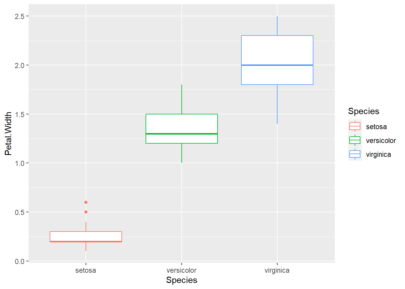
# 法一
iris.lm <- lm(Petal.Width~Species, data = iris)
iris.anova <- anova(iris.lm)
iris.anova
#> Analysis of Variance Table
#>
#> Response: Petal.Width
#> Df Sum Sq Mean Sq F value Pr(>F)
#> Species 2 80.413 40.207 960.01 < 2.2e-16 ***
#> Residuals 147 6.157 0.042
#> ---
#> Signif. codes: 0 '***' 0.001 '**' 0.01 '*' 0.05 '.' 0.1 ' ' 1# 法二
aov.method2 <- aov(Petal.Width~Species, data = iris)
summary(aov.method2)#> Df Sum Sq Mean Sq F value Pr(>F)
#> Species 2 80.41 40.21 960 <2e-16 ***
#> Residuals 147 6.16 0.04
#> ---
#> Signif. codes: 0 '***' 0.001 '**' 0.01 '*' 0.05 '.' 0.1 ' ' 1Species 總共有三個類別。計算如下:
Df
3 - 1#> [1] 2Sum Square
df1 <- iris %>%
  select(Species, Petal.Width) %>%
  group_by(Species) %>%
  summarise(mean = mean(Petal.Width), # 每個類別的平均值
            sqare_error = sum((Petal.Width - mean) ^ 2))
df1
#> # A tibble: 3 x 3
#> Species mean sqare_error
#> * <fct> <dbl> <dbl>
#> 1 setosa 0.246 0.544
#> 2 versicolor 1.33 1.92
#> 3 virginica 2.03 3.70sum((df1$mean - mean(df1$mean)) ^ 2) * 50#> [1] 80.41333# 同理
# var() 樣本變異數
var(df1$mean) * (3 - 1) * 50#> [1] 80.41333# sd() 樣本標準差
sd(df1$mean) ** 2 * (3 - 1) * 50#> [1] 80.41333Mean Square
# Sum sq / Df
80.413 / 2
#> [1] 40.2065Residuals 的計算如下:
Df
3 * (50 - 1)#> [1] 147Sum Square
sum(df1$sqare_error)#> [1] 6.1566Mean Square
# Sum sq / Df
6.157 / 147
#> [1] 0.04188435F value 計算如下:
40.207 / 0.042 # 誤差大#> [1] 957.3095(80.413 / 2) / (6.157 / 147) # 誤差小#> [1] 959.9408SSB <- sum((df1$mean - mean(df1$mean)) ^ 2) * 50
SSW <- sum(df1$sqare_error)
(SSB / 2) / (SSW / 147) # 誤差更小#> [1] 960.0071F 分配的形狀:
x <- rf(10000, 2, 147)
y <- df(x, 2, 147)
plot(x, y)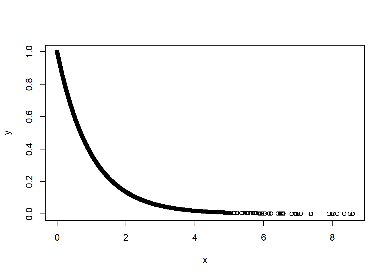
從上圖可以看出 F-value 大的時候,機率接近 0。因此 \(Pr(>F) < 2.2e-16\)
1 - pf(960.01, df1 = 2, df2 = 147) #> [1] 0Two-Way ANOVA
參考上課講義的題目,我們可以自行輸入資料:
driver <- c("Hamilton", "Bottas", "Verstappen", "Leclerc", "Vettle")
data <- tibble(driver = driver,
               A = c(18, 16, 21, 23, 25),
               B = c(17, 23, 21, 22, 24),
               C = c(21, 23, 26, 29, 28),
               D = c(22, 22, 22, 25, 28))

data
#> # A tibble: 5 x 5
#> driver A B C D
#> <chr> <dbl> <dbl> <dbl> <dbl>
#> 1 Hamilton 18 17 21 22
#> 2 Bottas 16 23 23 22
#> 3 Verstappen 21 21 26 22
#> 4 Leclerc 23 22 29 25
#> 5 Vettle 25 24 28 28資料需要做轉換才有辦法做分析。
data2 <- data %>%
  gather(-driver, key = "road", value = "time")

data2
#> # A tibble: 20 x 3
#> driver road time
#> <chr> <chr> <dbl>
#> 1 Hamilton A 18
#> 2 Bottas A 16
#> 3 Verstappen A 21
#> 4 Leclerc A 23
#> 5 Vettle A 25
#> 6 Hamilton B 17
#> 7 Bottas B 23
#> 8 Verstappen B 21
#> 9 Leclerc B 22
#> 10 Vettle B 24
#> 11 Hamilton C 21
#> 12 Bottas C 23
#> 13 Verstappen C 26
#> 14 Leclerc C 29
#> 15 Vettle C 28
#> 16 Hamilton D 22
#> 17 Bottas D 22
#> 18 Verstappen D 22
#> 19 Leclerc D 25
#> 20 Vettle D 28可以從列聯表看出每個項目只有一個樣本。
table(data2$road, data2$driver)#>
#> Bottas Hamilton Leclerc Verstappen Vettle
#> A 1 1 1 1 1
#> B 1 1 1 1 1
#> C 1 1 1 1 1
#> D 1 1 1 1 1因為每個項目只有一個樣本,所以使用 geom_point() 畫圖,如果多於一個樣本,畫 geom_boxplot() 更為合適。
ggplot(data2, aes(road, time, color = driver)) +
  geom_point()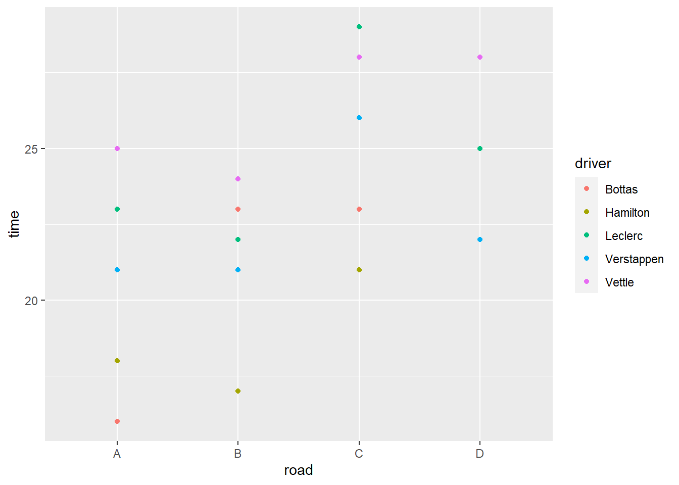
以下示範三種方法的程式碼:
# 法一
two.way.anova.1 <- lm(time ~ road + driver, data = data2)
twa.1 <- anova(two.way.anova.1)

# 法二
two.way.anova.2 <- aov(time ~ road + driver, data = data2)
summary(two.way.anova.2)

# 法三
two.way.anova.3 <- lm(data2$time ~ data2$road + data2$driver)
anova(two.way.anova.3)
以下可以觀察到三種作法都會得到相同的結果,當然細心的同學會說小數點後取的位數稍有不同。
法一: lm() 搭配 anova(),指定資料 data = data2 的寫法。
two.way.anova.1 <- lm(time ~ road + driver, data = data2)
twa.1 <- anova(two.way.anova.1)
twa.1$Df
#> [1] 3 4 12twa.1$`Sum Sq`#> [1] 72.8 119.7 36.7twa.1$`Mean Sq`#> [1] 24.266667 29.925000 3.058333twa.1$`F value`#> [1] 7.934605 9.784741 NAtwa.1$`Pr(>F)`#> [1] 0.0035079132 0.0009335737 NA法二: aov() 搭配 summary(),指定資料 data = data2 的寫法。
two.way.anova.2 <- aov(time ~ road + driver, data = data2)
summary(two.way.anova.2)
#> Df Sum Sq Mean Sq F value Pr(>F)
#> road 3 72.8 24.267 7.935 0.003508 **
#> driver 4 119.7 29.925 9.785 0.000934 ***
#> Residuals 12 36.7 3.058
#> ---
#> Signif. codes: 0 '***' 0.001 '**' 0.01 '*' 0.05 '.' 0.1 ' ' 1法三: lm() 搭配 anova(),不指定資料,變數取值的寫法。
two.way.anova.3 <- lm(data2$time ~ data2$road + data2$driver)
anova(two.way.anova.3)
#> Analysis of Variance Table
#>
#> Response: data2$time
#> Df Sum Sq Mean Sq F value Pr(>F)
#> data2$road 3 72.8 24.2667 7.9346 0.0035079 **
#> data2$driver 4 119.7 29.9250 9.7847 0.0009336 ***
#> Residuals 12 36.7 3.0583
#> ---
#> Signif. codes: 0 '***' 0.001 '**' 0.01 '*' 0.05 '.' 0.1 ' ' 1考慮交互作用
注意,這裡的資料與前面不同。
#交互作用
driver <- c("Hamilton", "Bottas", "Verstappen", "Leclerc", "Vettle")
data.int <- tibble(driver = factor(rep(driver, each = 3), level = driver),
                   A = c(18, 15, 21, 16, 19, 13, 21, 19, 14, 23, 21, 25, 25, 24, 26),
                   B = c(17, 14, 20, 23, 19, 25, 21, 23, 25, 22, 24, 20, 24, 25, 23),
                   C = c(21, 20, 22, 23, 24, 22, 26, 24, 28, 29, 30, 28, 28, 29, 27),
                   D = c(22, 19, 25, 22, 20, 24, 22, 24, 20, 25, 20, 26, 28, 30, 26))

data.int
#> # A tibble: 15 x 5
#> driver A B C D
#> <fct> <dbl> <dbl> <dbl> <dbl>
#> 1 Hamilton 18 17 21 22
#> 2 Hamilton 15 14 20 19
#> 3 Hamilton 21 20 22 25
#> 4 Bottas 16 23 23 22
#> 5 Bottas 19 19 24 20
#> 6 Bottas 13 25 22 24
#> 7 Verstappen 21 21 26 22
#> 8 Verstappen 19 23 24 24
#> 9 Verstappen 14 25 28 20
#> 10 Leclerc 23 22 29 25
#> 11 Leclerc 21 24 30 20
#> 12 Leclerc 25 20 28 26
#> 13 Vettle 25 24 28 28
#> 14 Vettle 24 25 29 30
#> 15 Vettle 26 23 27 26data2.int <- data.int %>%
gather(-driver, key = "road", value = "time")
data2.int#> # A tibble: 60 x 3
#> driver road time
#> <fct> <chr> <dbl>
#> 1 Hamilton A 18
#> 2 Hamilton A 15
#> 3 Hamilton A 21
#> 4 Bottas A 16
#> 5 Bottas A 19
#> 6 Bottas A 13
#> 7 Verstappen A 21
#> 8 Verstappen A 19
#> 9 Verstappen A 14
#> 10 Leclerc A 23
#> # ... with 50 more rows我們先計算路線平均時間,駕駛平均時間以及總平均時間。
# 路線平均
mfr <- data2.int %>%
  group_by(road) %>%
  summarise(means_for_route = mean(time))

mfr
#> # A tibble: 4 x 2
#> road means_for_route
#> * <chr> <dbl>
#> 1 A 20
#> 2 B 21.7
#> 3 C 25.4
#> 4 D 23.5# 駕駛平均
mfd <- data2.int %>%
group_by(driver) %>%
summarise(means_for_driver = mean(time))
mfd#> # A tibble: 5 x 2
#> driver means_for_driver
#> * <fct> <dbl>
#> 1 Hamilton 19.5
#> 2 Bottas 20.8
#> 3 Verstappen 22.2
#> 4 Leclerc 24.4
#> 5 Vettle 26.2# 總平均
mean(data2.int$time)#> [1] 22.65如果用列連表的形式,可以看出每位駕駛在每條路線都進行三次實驗。
table(data2.int$road, data2.int$driver)#>
#> Hamilton Bottas Verstappen Leclerc Vettle
#> A 3 3 3 3 3
#> B 3 3 3 3 3
#> C 3 3 3 3 3
#> D 3 3 3 3 3接著我們畫交互作用,也就是依照每位駕駛在每條路線的平均時間。
# 畫圖
data2.int %>%
  group_by(driver, road) %>%
  summarise(time = mean(time)) %>%
  ggplot(aes(road, time, color = driver)) +
  geom_point() +
  geom_line(aes(group = driver))
#> `summarise()` has grouped output by 'driver'. You can override using the `.groups` argument.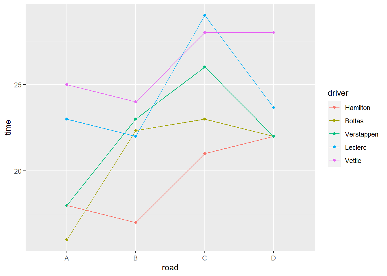
考慮交互作用的假設檢定如下:
\[ \begin{aligned} \left\{ \begin{array}{ll} H_0: 駕駛與路線之間沒有交互作用\\ H_1: 駕駛與路線之間存在交互作用 \end{array} \right. \end{aligned} \]
考慮交互作用的 two-way ANOVA 在 formula 有兩種寫法:
一種是把 + 改成 *,例如 time ~ road * driver;
另一種是 : 連接兩因子,例如 time ~ road + driver + road:driver。
# two-way ANOVA, consider interaction
two.way.anova.interaction <-
  aov(time ~ road * driver, data = data2.int)
twa.int <- summary(two.way.anova.interaction)
twa.int
#> Df Sum Sq Mean Sq F value Pr(>F)
#> road 3 245.0 81.66 15.908 5.84e-07 ***
#> driver 4 353.6 88.39 17.219 2.74e-08 ***
#> road:driver 12 125.8 10.48 2.042 0.0456 *
#> Residuals 40 205.3 5.13
#> ---
#> Signif. codes: 0 '***' 0.001 '**' 0.01 '*' 0.05 '.' 0.1 ' ' 1假如不拒絕虛無假設,可驗證兩因子個別的影響,回到 one-way ANOVA。
\[ \begin{aligned} \left\{ \begin{array}{ll} H_0: 駕駛的平均時間完全相同\\ H_1: 駕駛的平均時間不全相同 \end{array} \right. \end{aligned} \]
# 路線 A
data2.int %>%
  filter(road == "A") %>%
  aov(time ~ driver, data = .) %>%
  summary()
#> Df Sum Sq Mean Sq F value Pr(>F)
#> driver 4 174 43.5 6.042 0.00974 **
#> Residuals 10 72 7.2
#> ---
#> Signif. codes: 0 '***' 0.001 '**' 0.01 '*' 0.05 '.' 0.1 ' ' 1# 路線 B
data2.int %>%
filter(road == "B") %>%
aov(time ~ driver, data = .) %>%
summary()#> Df Sum Sq Mean Sq F value Pr(>F)
#> driver 4 88.67 22.167 4.055 0.033 *
#> Residuals 10 54.67 5.467
#> ---
#> Signif. codes: 0 '***' 0.001 '**' 0.01 '*' 0.05 '.' 0.1 ' ' 1# 同理,自行練習路線 C 和 D\[ \begin{aligned} \left\{ \begin{array}{ll} H_0: 路線的平均時間完全相同\\ H_1: 路線的平均時間不全相同 \end{array} \right. \end{aligned} \]
# 駕駛 Hamilton
data2.int %>%
  filter(driver == "Hamilton") %>%
  aov(time ~ road, data = .) %>%
  summary()
#> Df Sum Sq Mean Sq F value Pr(>F)
#> road 3 51 17 2.429 0.14
#> Residuals 8 56 7# 同理,自行練習其他駕駛作業
使用手邊的資料進行 ANOVA 分析。 One-way 和 Two-way 都做一題,練習看看。